
Hi!
Until the end of 2025, I worked as an assistant for RF (Radio Frequency) engineers. It can be a very theoretical field, so I decided to do some hands-on projects at home! I wondered: Could I reverse-engineer a simple toy car remote and figure out how it communicates with the car? It turns out, it’s possible! And you can do much more, too!
Demo #
I was able to play a computer racing game with a toy car remote!
Overview
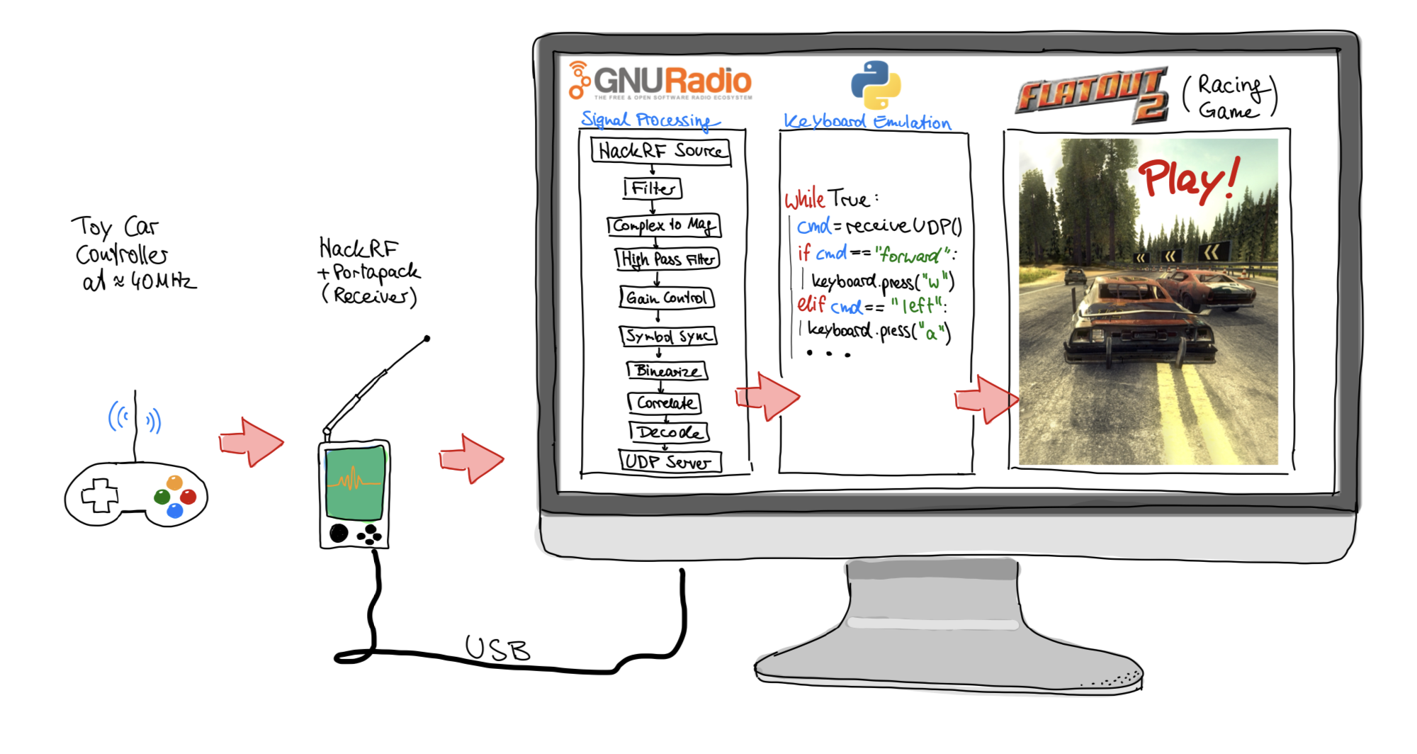
This is the system I created – I’ll explain it in this article and describe the process of reverse-engineering the remote radio connection and developing a custom, real-time decoder. Although this might sound intimidating, I want to make the topic approachable by avoiding using a lot of technical terms and relying on plenty of photos and videos.
Introduction #
Thanks to my time at university, I already have some background in signal processing, communication engineering and related fields. I read about the HackRF and GNU Radio on the internet, so I decided to give it a try. I bought a HackRF and a toy car from eBay Kleinanzeigen (the German equivalent of Craigslist), so I had something to start with!
Let’s start small by looking at the toy car.
Lightning McQueen! (The actual toy car) #

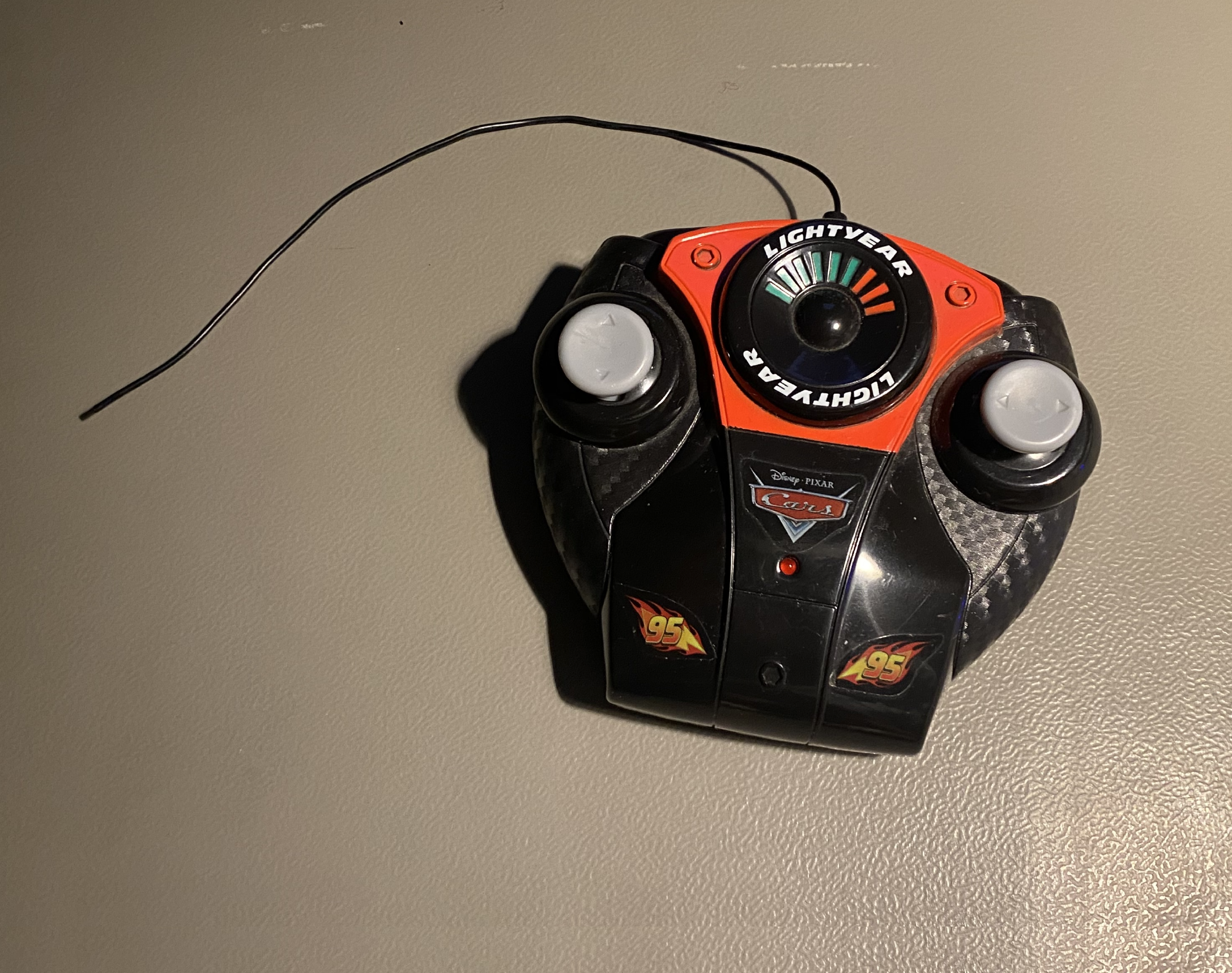
The toy car works, yay! However, I did need to replace the batteries.
Introduction to the radio world #
So let’s start simple - what are radio signals about?
When alternating the current in a wire multiple millions of times per second, the electric and magnetic field around the wire start to interact with each other and propagate (travel) away from the wire into the air. We call the wire an antenna, and it transmits at a frequency. We usually do this in Megahertz (MHz), where 1 MHz means one million cycles per second.
Now, as these electromagnetic waves propagate through the room, they will bump into other wires. When they do, they create a tiny voltage inside those wires at the exact same frequency, which we then measure. By using electronic components like amplifiers and filters, we can make this tiny signal usable.
The cool thing is that one can choose exactly what frequency to transmit and receive on! And there are a massive number of different frequencies – ranging from a few MHz to like 60 GHz. Here is a short overview:
- 1 kHz - 1,000 periods per second
- 1 MHz - 1,000,000 periods per second
- 1 GHz - 1,000,000,000 periods per second
- 1 THz - 1,000,000,000,000 periods per second
Now the complete collection of all frequencies is called the “frequency spectrum”. If you need a specific range of frequencies for your project, you use a frequency “band”.
Some frequency examples:
- Ca. 100 MHz: Typical kitchen FM radio music
- Ca. 150 MHz: Amateur (HAM) radio people talking to each other
- 2.4GHz: Wi-Fi, Bluetooth, Microwave ovens
- 5 GHz: Faster Wi-Fi
Now you might think, electro-magnetic waves can only be used for communication, but there are many other uses! For example:
- Ca. 50kHz: Wireless charging (at this low frequency, it relies mostly on magnetic coupling effects rather than true radiating radio frequencies)
- Ca. 60 GHz: Radar applications that measure distance and speed.
- Ca. 550 THz: Visible, Green light! (Light is an electromagnetic wave too!)
When engineers develop radio communication systems, there are a lot of tasks to be done:
- Choose frequency
- Develop radio components: Antenna (physical dimensions, material), Amplifiers, filters
- Develop radio modulation: Decide which property of the radio signal actually carry information
- Develop radio protocols: Figure out rules who should transmit and receive at which exact time, so that everyone’s signals don’t crash (interfere) into each other.
- Develop software: Make this technology accessible so that software developers can include it in their products easily!
What is a HackRF #
My personal goal is to understand and model the radio connection between the car and the remote. To get started tinkering with radio communication, a device like a HackRF is needed.
A HackRF is like a Swiss Army knife for receiving and also transmitting radio signals between 1 MHz and 6 GHz. It can be used to take part in amateur radio conversation, know what planes are over your head, hack toys and more. A friend of mine uses the HackRF to receive and decode images transmitted by satellites. In radio/RF engineering world, it’s called a software defined radio, in short SDR. And yes, like any tool, this device can be used for illegal stuff too - like hacking car keyfob signals to break into cars. I will refrain from this and use the device only for receiving remote commands for educational purposes.
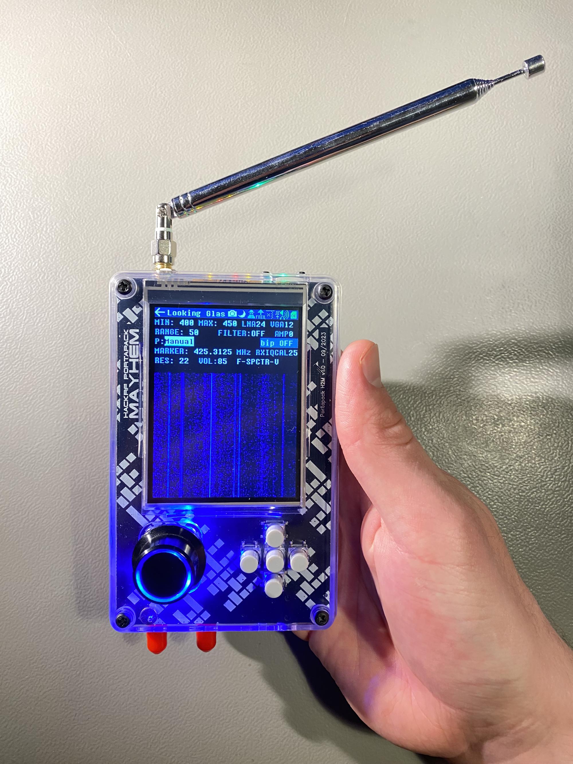
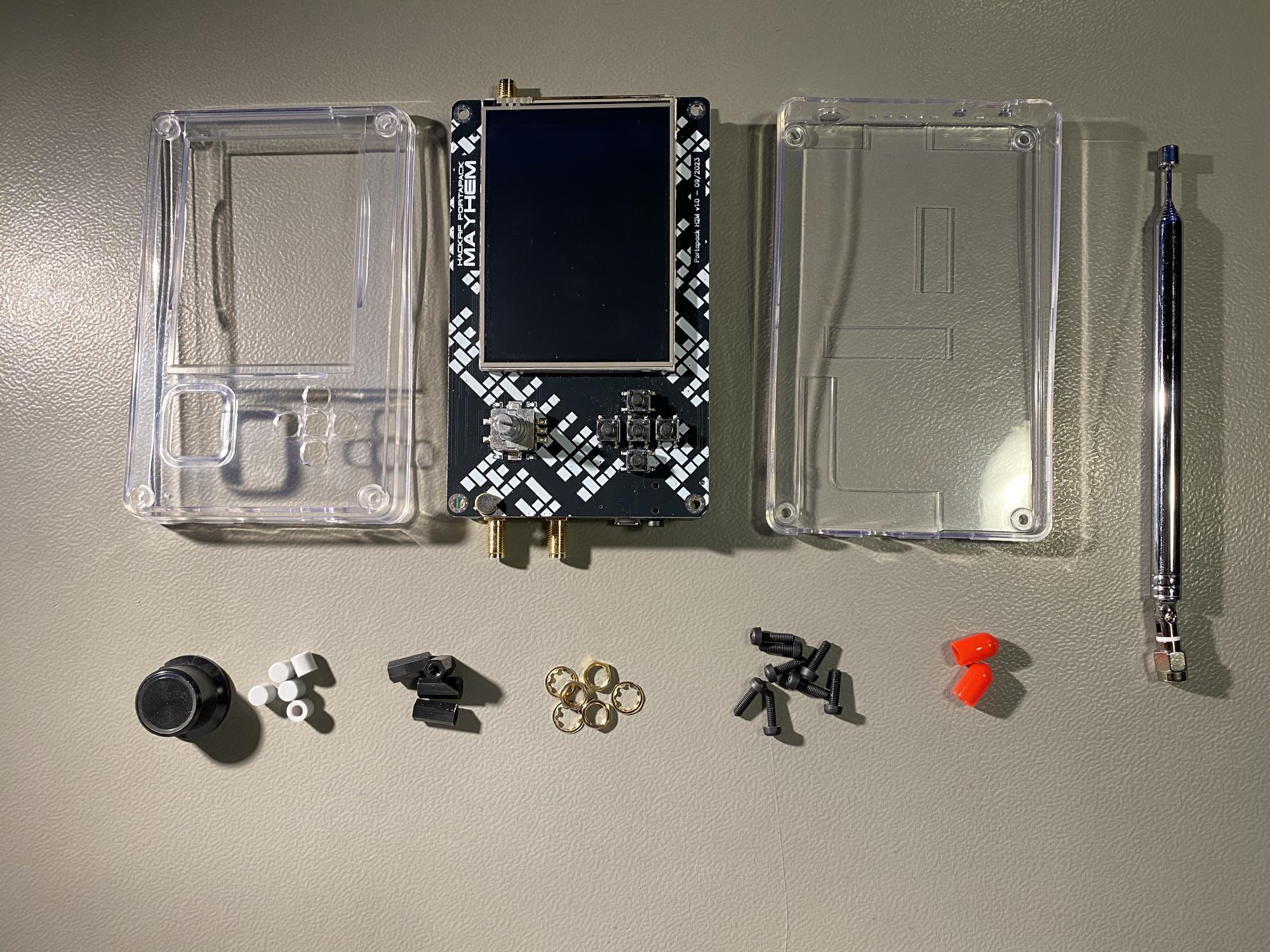
Actually, the HackRF is just a green PCB inside the device I am holding in my hand. What you see is an extension of the HackRF called “Portapack” to make it portable! It adds the nice screen, buttons, battery and more. If you are interested in what the HackRF looks like without the extension, take a look at Attachment 1: The inside of the HackRF/Portapack.
Chapter 0: Let’s look more closely at the remote #
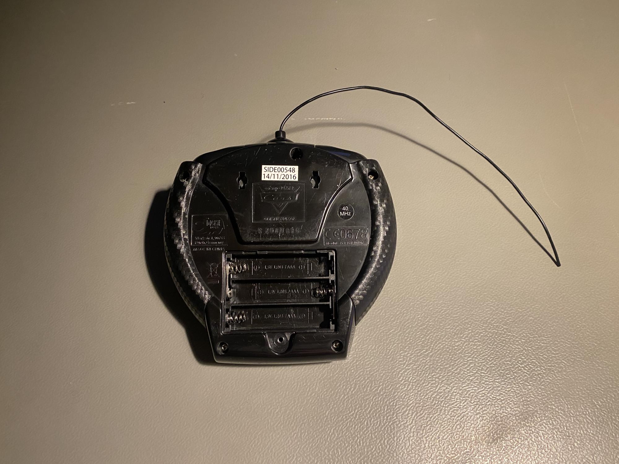
Do you spot the “40 MHz” label? Maybe that’s the frequency the remote is communicating on? If you are interested in what the disassembled car and remote look like, refer to attachment 2.
Chapter 1: Finding the toy car remote signal #
The first challenge is to find the remote signal. Now with the HackRF/Portapack, we can use the tool “Looking Glass”, which shows us the signal strength at all frequencies. Let’s tune to around 40 MHz!
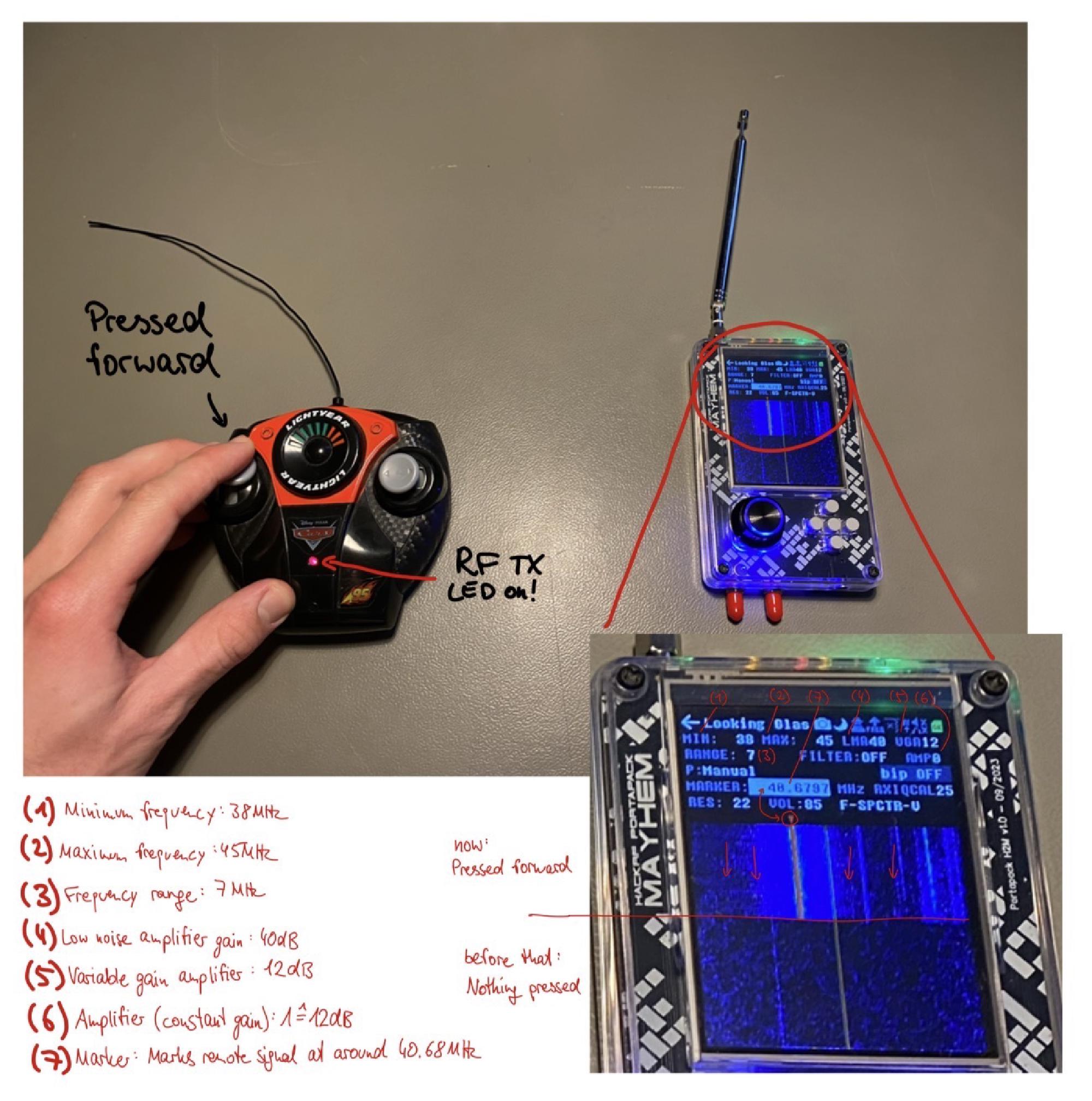
What did I do in Video 3 :
- Boot the HackRF/Portapack
- Open the Looking Glass App to find signals
- Select a frequency range that’s around 40MHz - to be specific: 38 MHz - 45 MHz
- Whenever we select a frequency span of less than 20MHz, then we see a bright vertical line exactly in the center of the screen. We just need to ignore this.
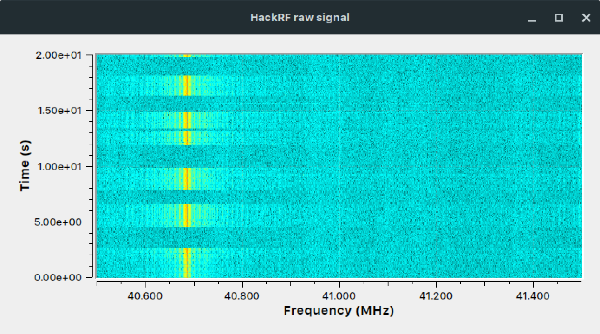
- When moving the joysticks, another bright vertical line appears on the screen, with some blue noise on the sides. That’s the signal! By the way: The display type is called a waterfall diagram. The frequencies are on the horizontal axis, time is on the vertical axis.
- The marker tool shows that the signal is not exactly 40MHz, its more between 40.6MHz and 40.7MHz (Actually, it’s 40.685MHz).
What’s exactly on the HackRF screen?
There are even more observations
- The signal is completely gone when not sending commands
- The frequency used seems to be always the same for every command
- It’s difficult to guess the type of modulation (which properties of the signal tell the commands like steering, accelerate and more)
Why did the manufacturer choose exactly 40.685 MHz?
Since radio frequencies are accessible to anybody and can be used for all kinds of communication applications and even more, it’s a highly valuable resource. The German Bundesnetzagentur has allocated specific frequency ranges/bands very precisely to different applications/companies. One can download a table with all the frequency allocations in Germany – on page 753, the important entry for us can be found:
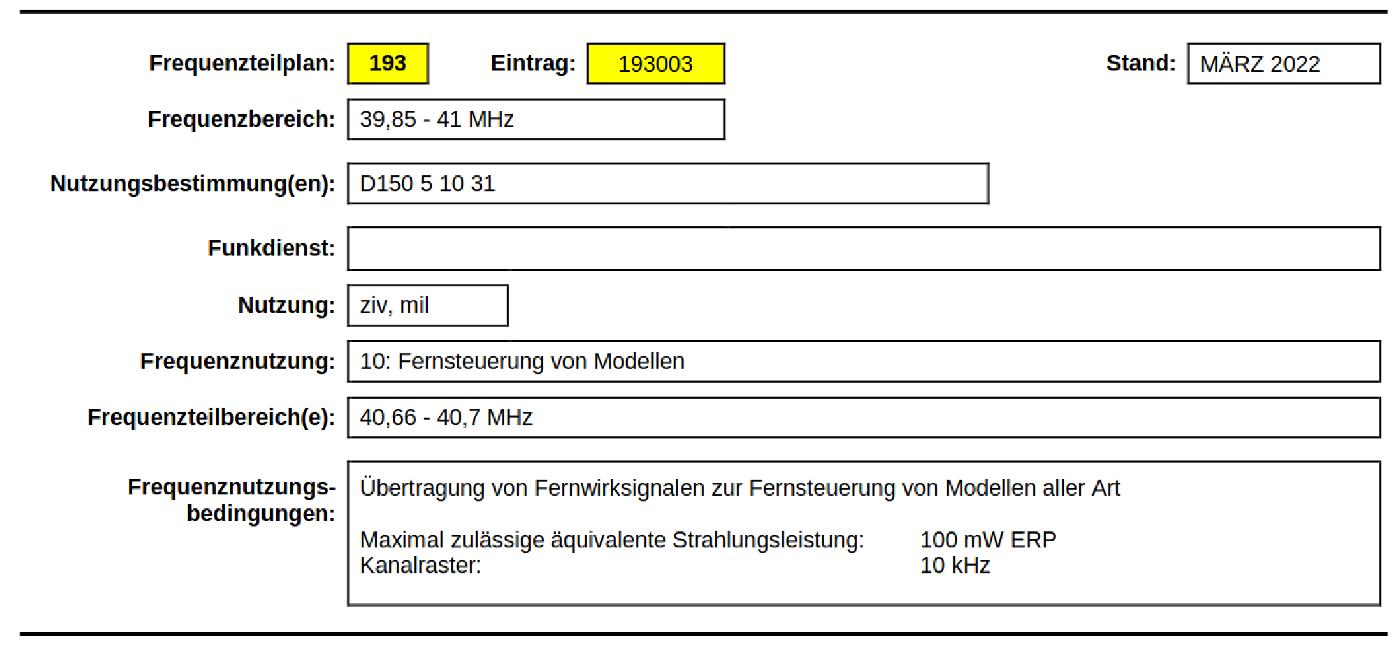
The frequency range 40,66 MHz to 40,7 MHz is specifically allocated for the remote models – like our toy car.
Chapter 2: Use GNU Radio companion to find the commands #
Connecting the HackRF to a computer allows for much more functionality. Instead of the Portapack extension processing the signal, now the computer does it with much more processing power and flexibility.
What is GNU Radio companion (GRC)?
The bundle GNU Radio and GNU Radio Companion (GRC) is a digital signal processing playground. It’s basically a tool kit with the following procedure:
- With the GNU Radio companion, complex decoder and transmitter flows can be designed by drag-and-dropping blocks (seen in figure 8)
- When clicking the play button:
- Python code is automatically generated and executed, which depends on the GNU Radio Python library
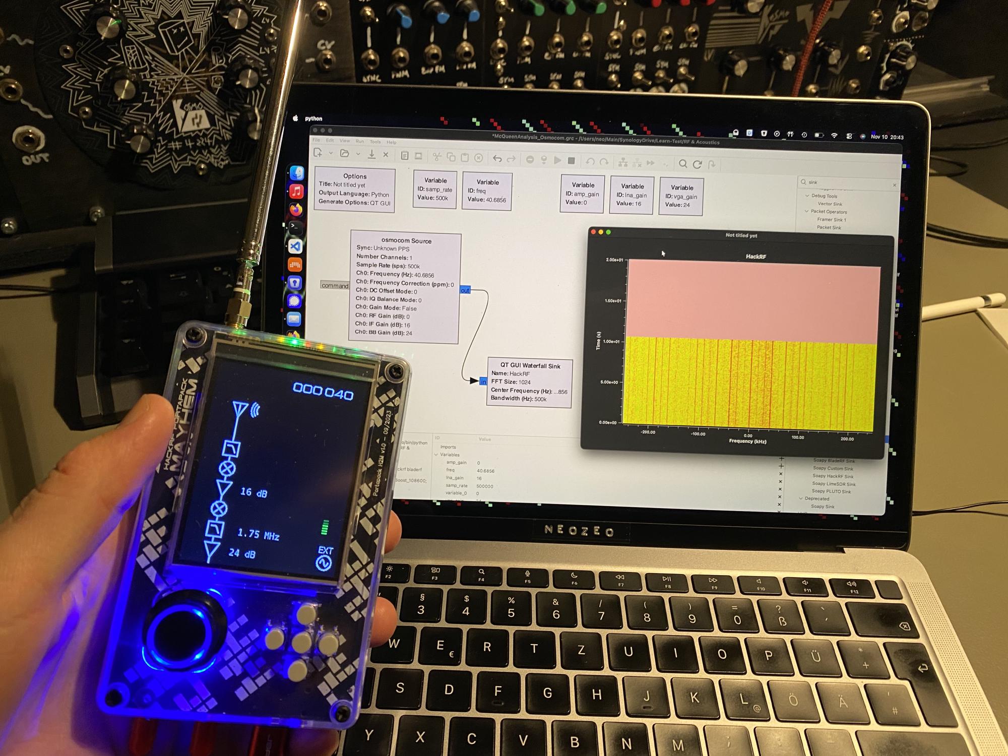
- Live graphs can be shown, like to be seen in figure 8 or 10.
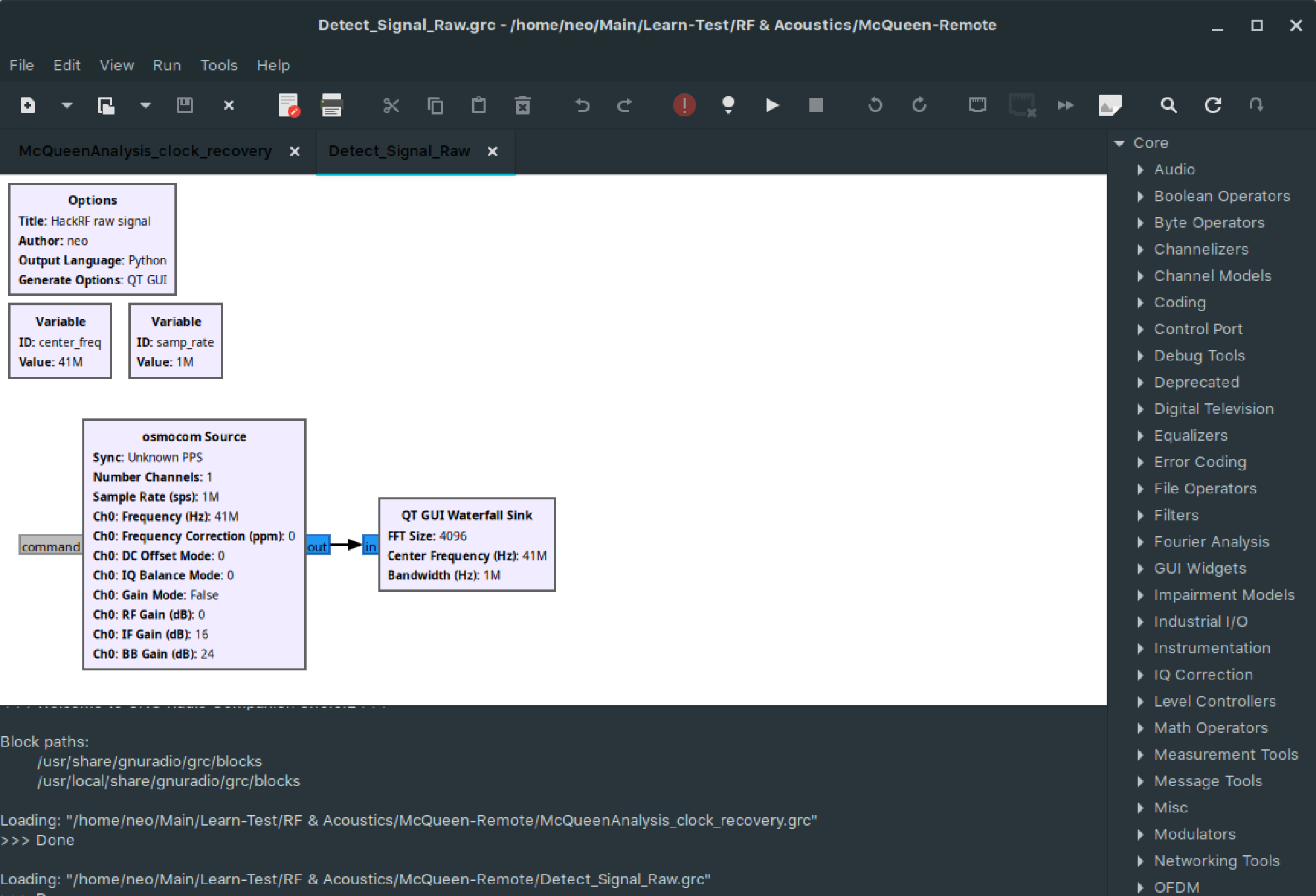
Let’s look on our receiver data flow in figure 9: Inside the white area in the center of the window, multiple blocks can be seen. The first, big block on the left, called “osmocom source”, is the HackRF signal source. The block on the right, called “QT GUI Waterfall Sink” is the receiver of the HackRF signal. When pressing play, the “QT GUI Waterfall Sink” block opens the window shown in figure 10. Both blocks can be configured with a lot of different parameters like sample rate, center frequency and more.
Now one could ask - why the hell should I use the complicated GNU Radio companion instead of the built-in functions on the HackRF/Portapack? Let’s compare:
When to use the integrated HackRF/Portapack functions
- When being on the go
- When only simple, common functionality is needed
- When starting out with an experiment
When to use GNU Radio companion
- For custom signal processing! We see later what it means.
- For a bigger screen and more graphs - with our new screen, we see the signal is exactly at 40.685 MHz
- Very complicated to get up and running though!
Chapter 3: Use GRC to find out more about the signal encoding #
Now comes the part, where we actually need a tool like GRC. With the signal recorded with the HackRF, we want to find out the signal-properties that tell us the command from the remote controller – aka what kind of modulation the remote controller uses! In university lectures like communication fundamentals, different modulation techniques are presented.
Let me present to you some common, very simple modulation techniques:
-
Amplitude modulation (AM)
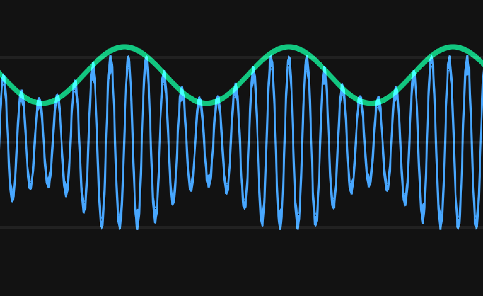
Figure 11: Amplitude modulation. Blue wave: Transmitted signal. Green wave: Actual information This is the simplest method: The amplitude (similar to the signal strength) actually tells us the information. In old radios, the AM was used to transmit music. And it probably was analog - meaning there was an infinite range of levels between a low and high amplitude. Now in digital communications, there are only certain amplitude levels:
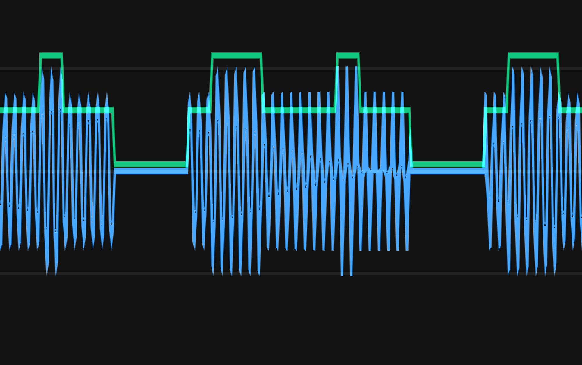
Figure 12: Amplitude shift keying modulation. Blue wave: Transmitted signal. Green wave: Actual information The most simple digital amplitude modulation is so-called On-Off-Keying – being like Morse code: There are only two amplitude levels: On or off!
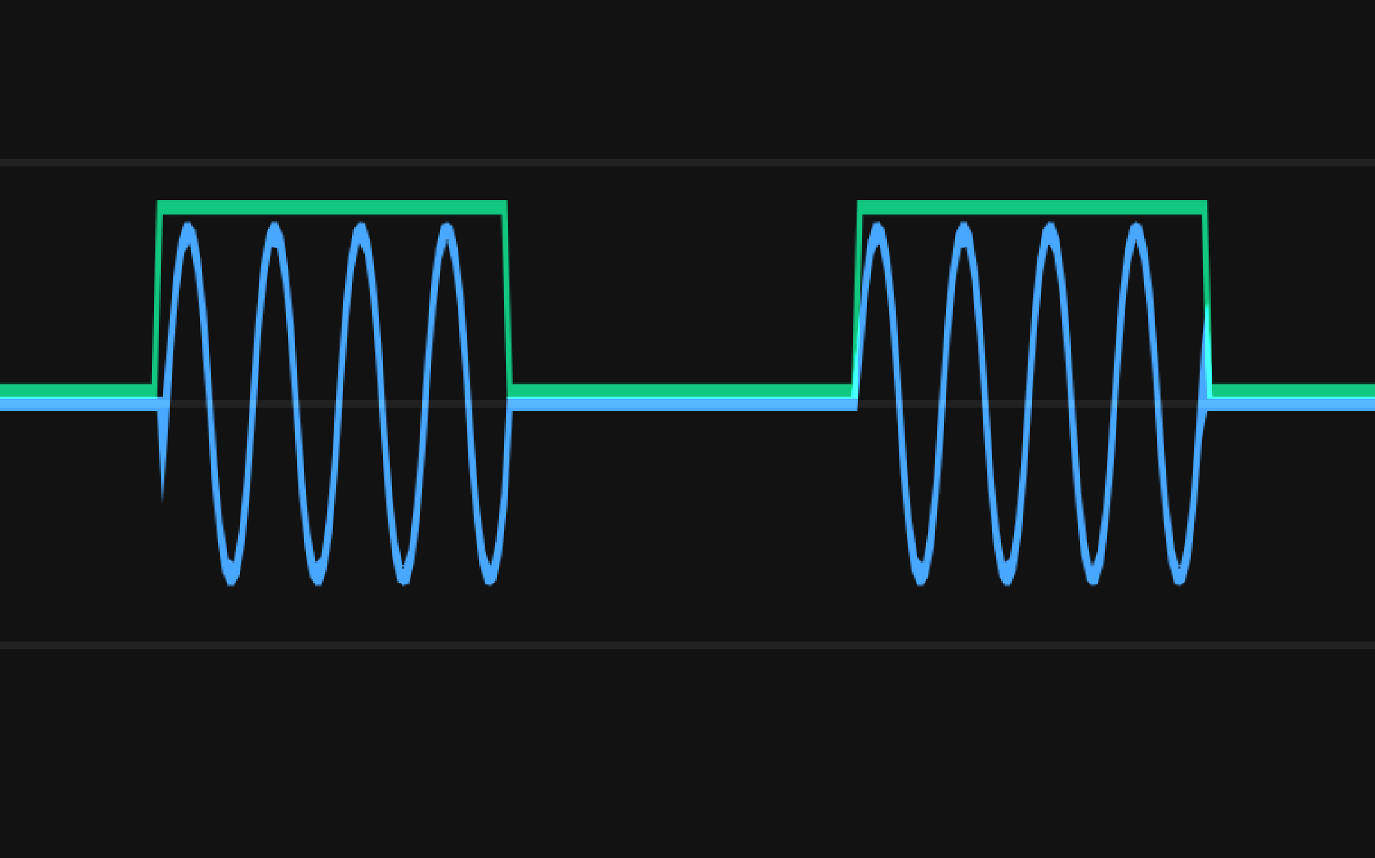
Figure 13: On-Off-Keying modulation. Blue wave: Transmitted signal. Green wave: Actual information -
Frequency modulation (FM)
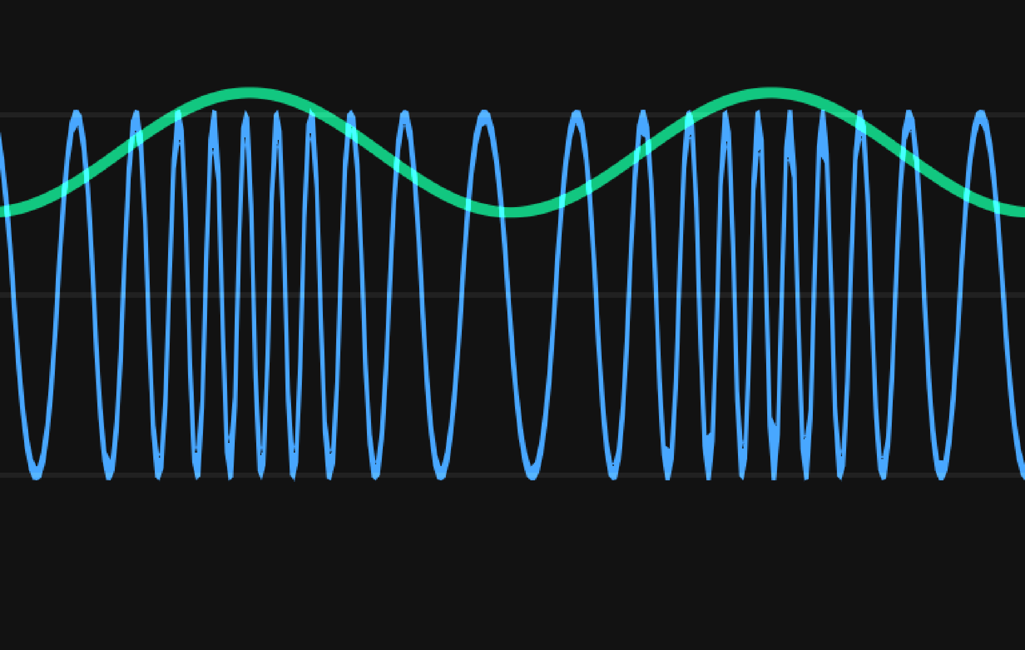
Figure 14: Frequency modulation. Blue wave: Transmitted signal. Green wave: Actual information Now in this method, we actually don’t vary the amplitude, but the frequency (very slightly). This can be observed by the receiver, which listens to a frequency range. Kitchen radios use FM since the 1970s. If we want to transmit digital information instead of sound, then so-called “frequency shift keying” can be used:
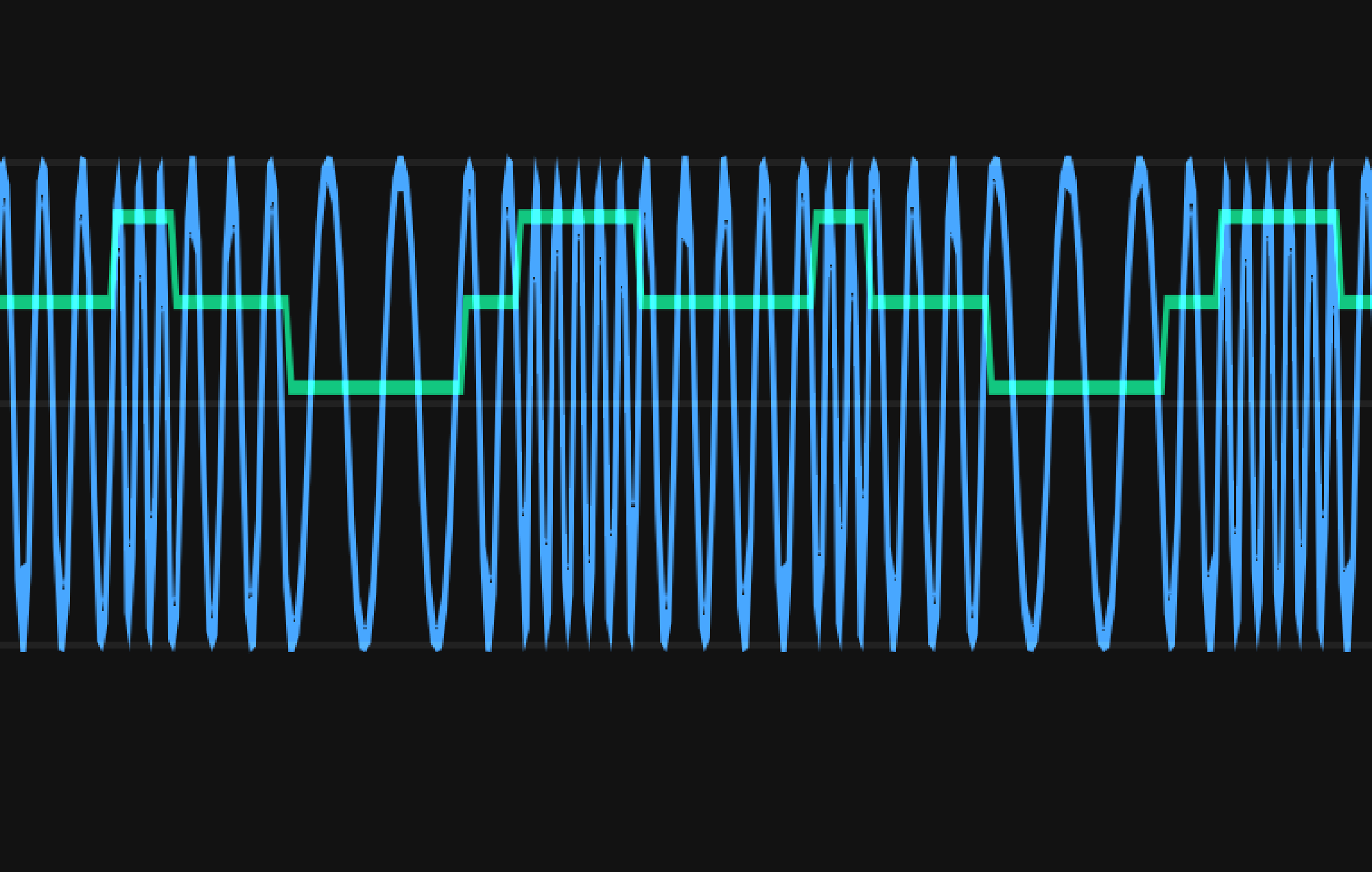
Figure 15: Frequency shift keying modulation. Blue wave: Transmitted signal. Green wave: Actual information -
Phase shift keying (PSK)
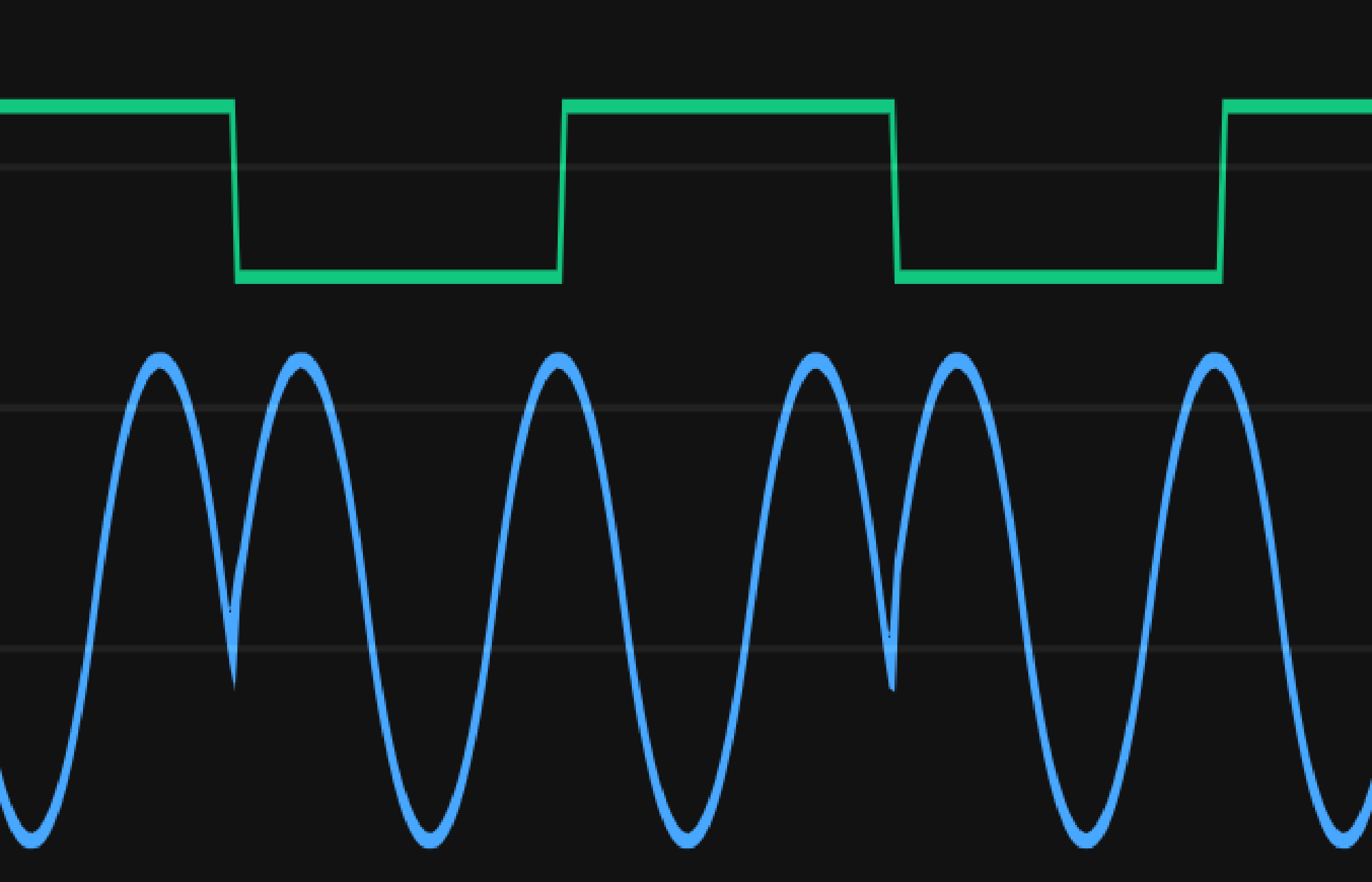
Figure 16: Phase shift keying modulation. Blue wave: Transmitted signal. Green wave: Actual information In this case, the frequency and amplitude stay the same, but the signal resets to the starting point sometimes, which transfers the information. This could also be used.
-
There are many more! Quadrature Amplitude modulation, Quadrature phase shift keying, etc.
What kind of modulation could our signal be?
Let’s compare the waterfall diagram of typical kitchen frequency-modulated radio signals with the one of the remote controller signal. I recorded both - all parameters are the same except the center frequency of the HackRF.
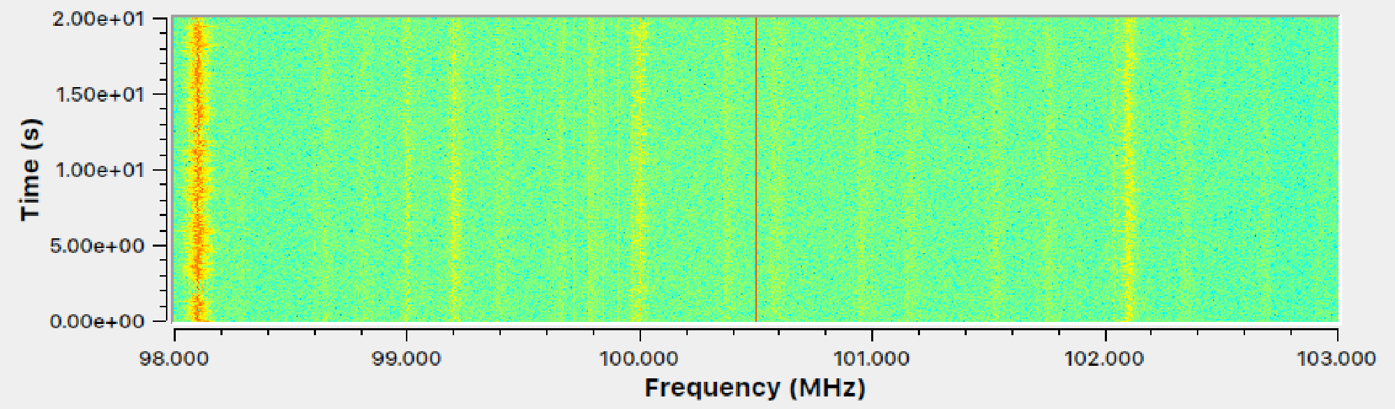
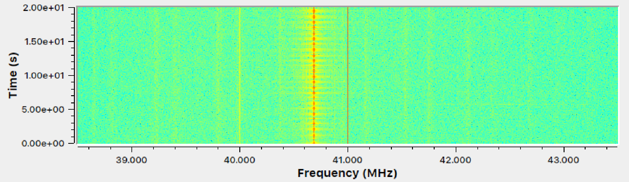
What do we observe?
- Many more signals in Figure 17 : In the waterfall graph, if we look closely, we see many signals displayed by yellow-ish vertical lines. The most dominant signal in Figure 17 being at ~98.1 MHz, the second to most dominant one at ~102.1 MHz. In the second graph, we see mostly one main signal – that’s our remote controller signal at 40.685 MHz.
- Perfect red line in the center: In both graphs, we have a deep red center line. We need to ignore it as it’s an artifact of the HackRF.
- The important point: The FM signals in Figure 17 seem to wobble around a specific center frequency, while our remote controller signal in Figure 18 is much more focussed at a single center frequency. Since the controller signal at 40.685 MHz basically doesn’t vary in frequency, we can assume it uses some kind of amplitude modulation!
Chapter 4: Another viewing angle of the signal to reveal the protocol #
Since we have the suspect amplitude modulation (AM), we can start building a receiver. Let’s look again at the amplitude modulation:
What we receive with the HackRF, is something like the blue wave. However, the green wave displays the amplitude – we want to get that green wave! The plan:
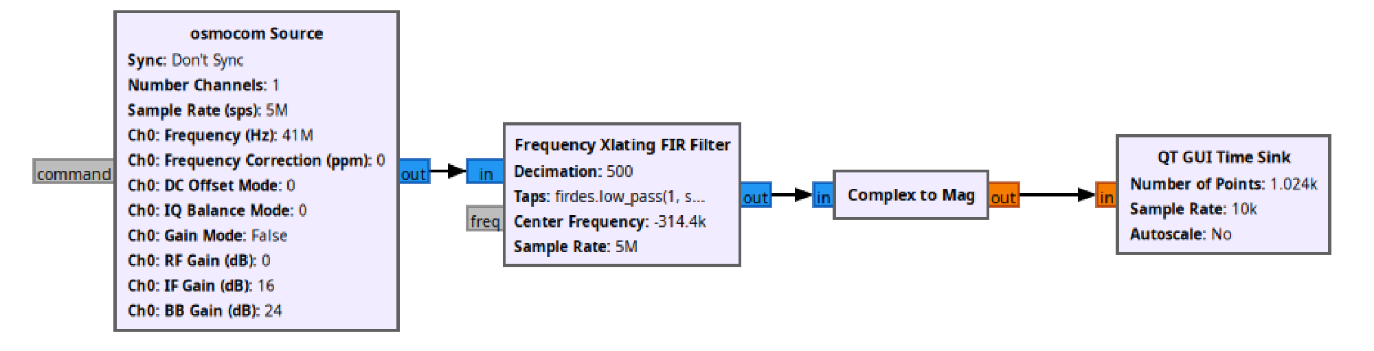
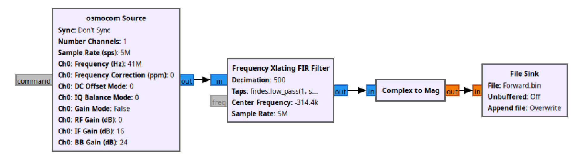
- Osmocom Source block: we receive signals at a center frequency of 41MHz and a span (aka band) of 5MHz (so we receive signals between 38.5 MHz and 43.5 MHz).
- Frequency Xlating FIR Filter block: Complicated block to select only our frequency of 40.685 MHz frequency range
- Complex to Mag block: Get the magnitude of our signal, which is essentially the same as the amplitude
- QT GUI Time Sink block: Just a live plot that displays the magnitude over time
The following graphs now show just the signal amplitude, which is the green wave in Figure 19 .
What do we observe?
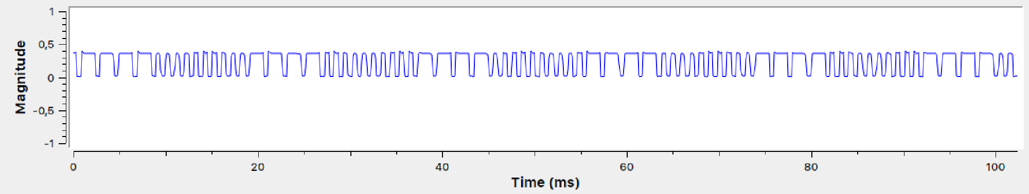
Wow! That looks promising! What is going on when trying another button?
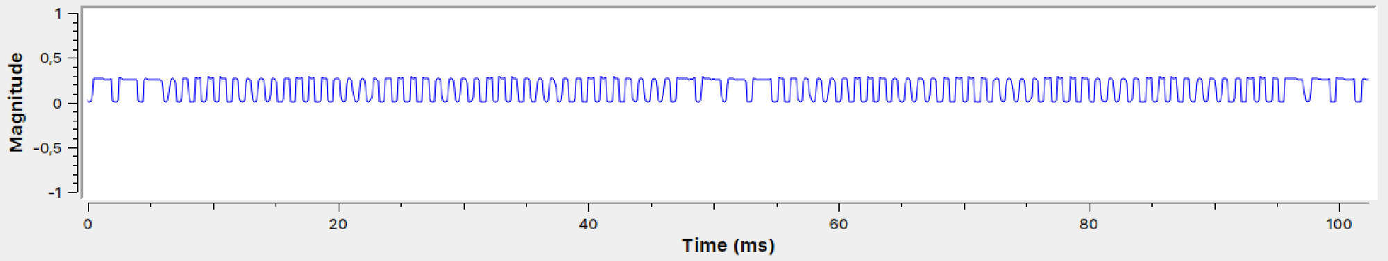
And when not pressing anything?
Okay, that’s pretty cool, huh? That delivers several new insights!
- There only seem to be two major amplitude levels. That means we have an OOK-type of amplitude modulation! (Either the signal is on, or off).
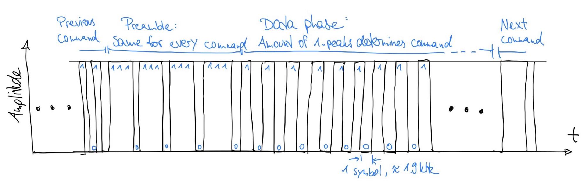
- If a key is continuously pressed, one can see a sequence of pulses that gets repeated. This sequence can be divided into two alternating phases:
- Phase 1 consists of four long pulses and is the same for every remote command. It could be a preamble to wake the toy car up!
- Phase 2 consists of short pulses – the number of which changes depending on the key pressed.
Here is a quick illustration on my thoughts:
I tried every command on the controller. Phase 1 is always the same, these are the pulse counts in phase 2:
| Command | Pulse Count |
|---|---|
| STOP | 4 |
| FORWARD | 10 |
| LEFT | 58 |
| RIGHT | 64 |
| BACKWARD | 40 |
| FORWARD_FULLSPEED | 22 |
| FORWARD_FULLSPEED_LEFT | 28 |
| FORWARD_FULLSPEED_RIGHT | 34 |
| BACKWARD_RIGHT | 46 |
| BACKWARD_LEFT | 52 |
Side-note: We need to hope the car does not do an initial hand-shake with the remote when they are turned on. Also, we hope, there is not a more intricate protocol involved, and the remote controller just repeats sending the commands to the car.
Chapter 5: Use Python to find out even more #
In the last chapter, we got a pretty good idea of the protocol system of the remote. It’s cool to be able to decode commands now by hand by looking at the graphs. But it would be even cooler to do the decoding automatically! Essentially, we want GRC to automatically detect the preambles in phase 1, then count the pulses in phase 2 and somehow match it to the commands.
Problem: For automatic detection of the preambles and the pulses afterwards, we need the frequency of how many times per second the magnitude flips to on or off. In communication engineering, we call that “symbol rate” - the number of events per second. To detect that, we can take a look at the frequency of the signal.
The plan: First, with the following GRC flow, we record the magnitude when a command is pressed continuously:
Second, we use a little vibe-coded Python-script:
- Open and parse the recording
- Do a “fourier transform” to get the frequencies of the signal
- Search for the frequency with the maximum magnitude
- Plot both the signal over time, and also its frequencies
- Mark the frequency with the maximum magnitude in the frequency plot
- Display the frequency also in the time plot by putting a red line after each period
The result:
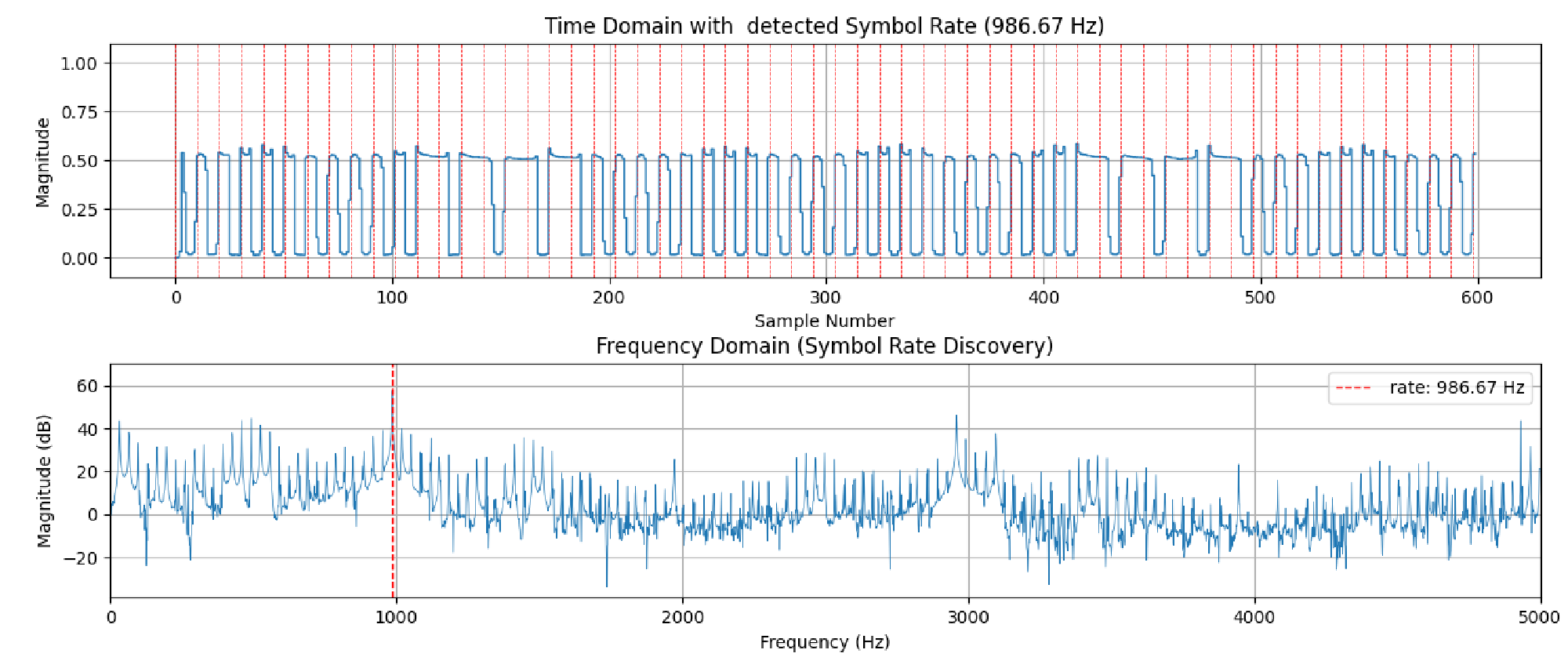
What do we observe? The frequency with the maximum magnitude is 989Hz. We can see a peak under the red line in the frequency domain plot. When looking in the time plot, we see one red line for every peak. However, that’s not what we want! We want the symbol rate to match the rate of magnitude on/off flips. However, this should double the frequency, around 1.9 kHz. Let’s plot this frequency too!
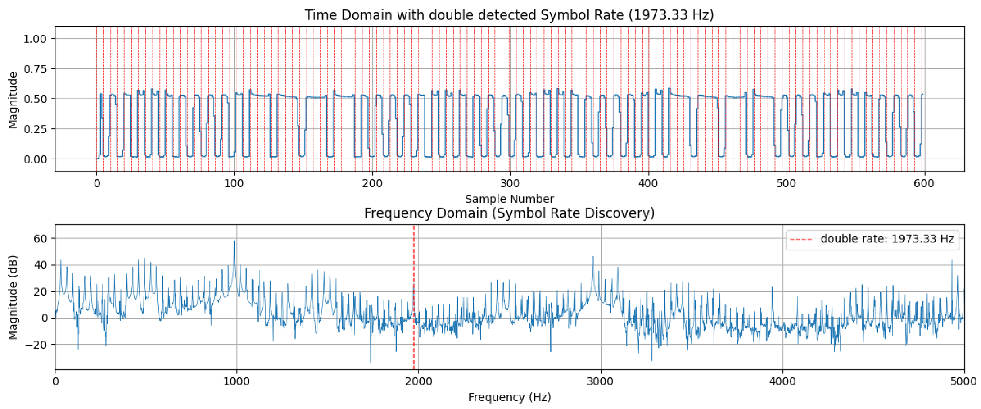
That’s looking much better, isn’t it? – The symbol rate really is at 1,973.33 Hz! We now have everything to build an automatic decoder as we know how often we need to look out for a flip in the amplitude.
Chapter 6: Use GRC to decode the commands in real-time #
We now found out everything we need to reverse-engineer the toy car receiver with GRC. I developed two iterations of decoders:
Decoder version 1 #
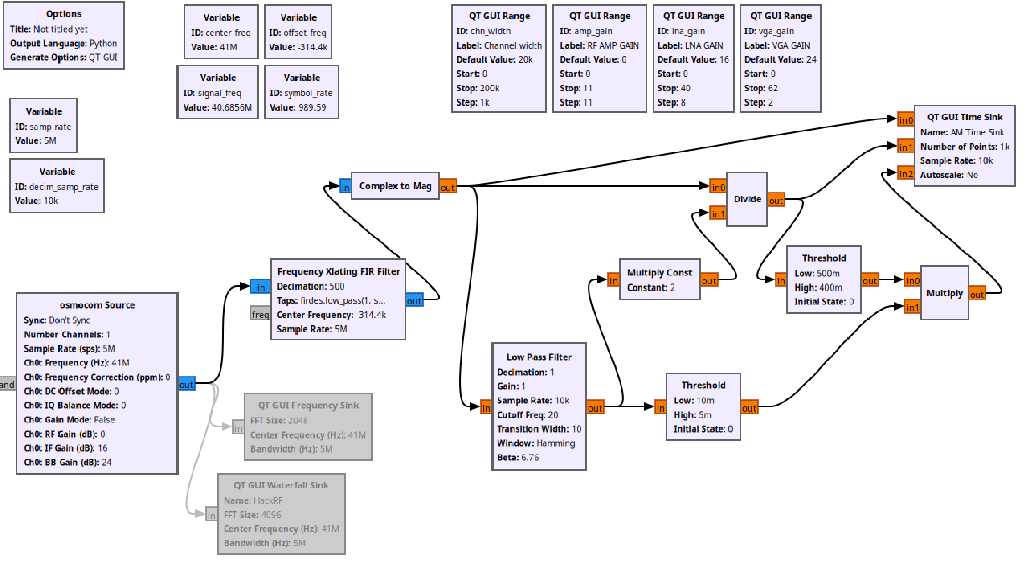
The signal chain consists of the following parts:
- Again: osmocom Source: HackRF signal source
- Again: Frequency Xlating FIR Filter block: Complicated block to select only our frequency of 40.685 MHz frequency range
- Again: Complex to Mag block: Get the magnitude of our signal, which is essentially the same as the amplitude
- Low pass filter, Multiply Const, etc.: VERY, very overcomplicated signal processing that should clean up the signal by extracting only ones and zeros. First, it’s an automatic signal gain control that results in the signal to always having an amplitude of one and second, it applies a threshold to the signal to get a binary signal that contains either ones or zeros.
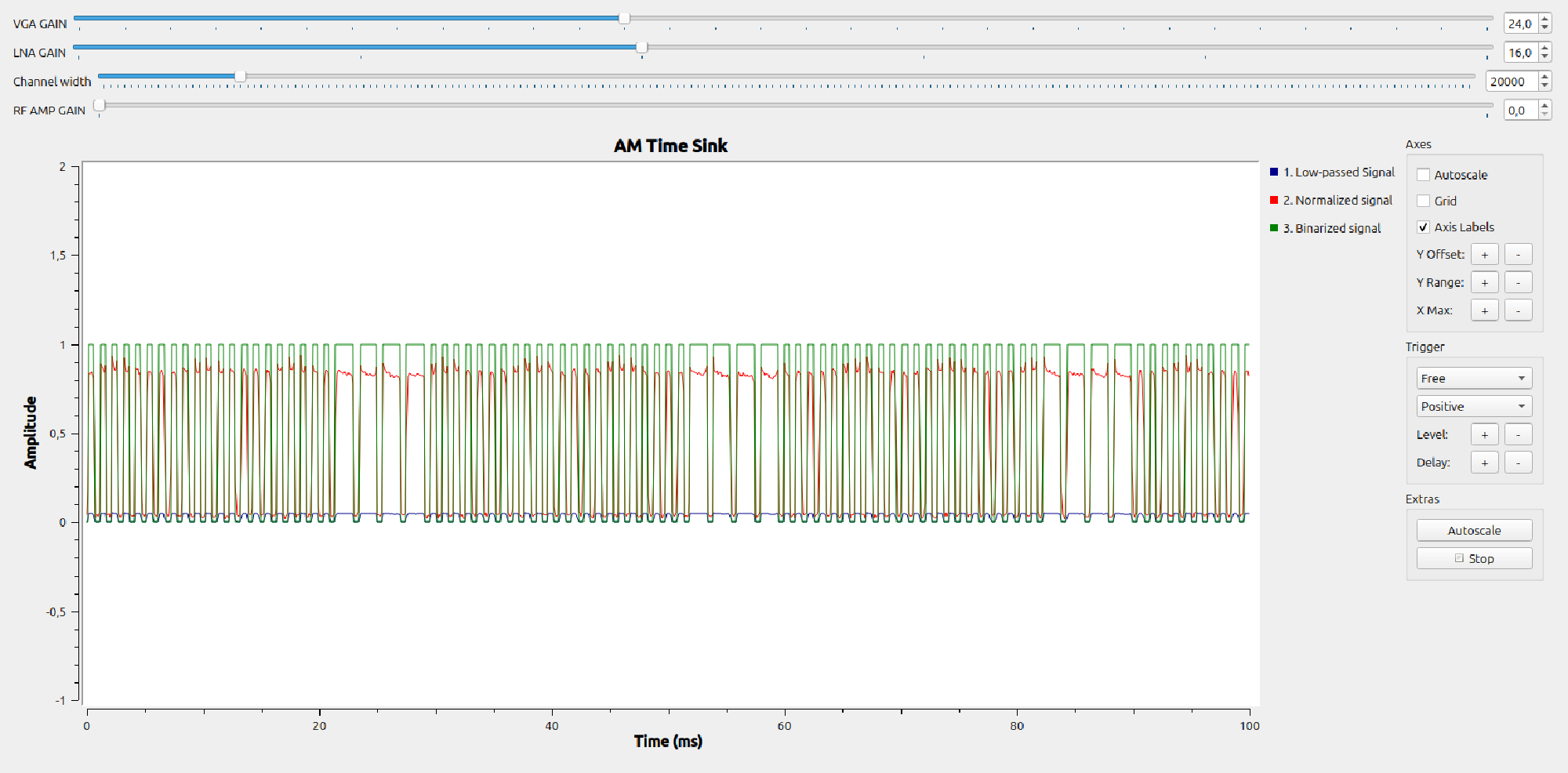
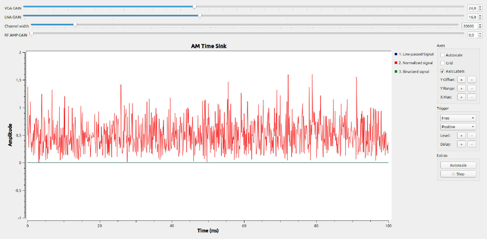
- QT GUI Time sink
- Raw, signal (very small amplitude)
- “Normalized” signal with amplitude being around one. It works as long as the distance between the remote controller and the HackRF is within 3 m.
- The binary signal which is either one or zeros.
This version still misses a lot of signal processing:
- Preamble detection & Pulse counting
- Matching pulse counts to commands
- Somehow simulate keyboard commands to play computer games
Live view
Decoder version 2 #
Although the first, naive path provided some insights, it is still not possible to really detect commands. This is why, I developed another signal chain:
General strategy for demodulation:
- Record signal amplitude like before
- High Pass filter: Center the amplitude signal vertically, so it’s zero on average.
- AGC: Instead of developing the automatic gain control myself, I used a pre-built block.
- QT GUI Time Sink: We all want to know what goes on in the signal chain to ensure it runs fine!
- Symbol Sync: This is a very important block - it uses the incoming signal to detect the important bit flips in our signal. It reduces (aka decimates) the recorded samples to only the few relevant ones.
- Binary slicer: Cleans the signal to be only ones or zeros. The output is pink since the signal data type now is single characters.
- Correlate Access Code - Tag: Searches continuously in the signal to find the access code (the pulses of phase one of the remote command).
- Char to float: Converts the signal back to floating-point numbers
- QT GUI Time Sink: We also want to see this signal!
- Command decoder: This is a custom, Python block, again, vibe-coded with AI:
- If the correlate access code - tag block indeed finds the phase 1 part of the signal:
- Count rising edges (being the short pulses of phase 2)
- Match the recorded pulse-count to the pulse-counts of existing commands
- Display the decoded command in the UI window
Live view
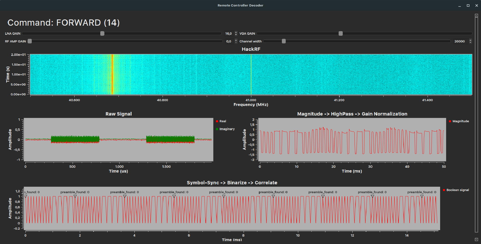
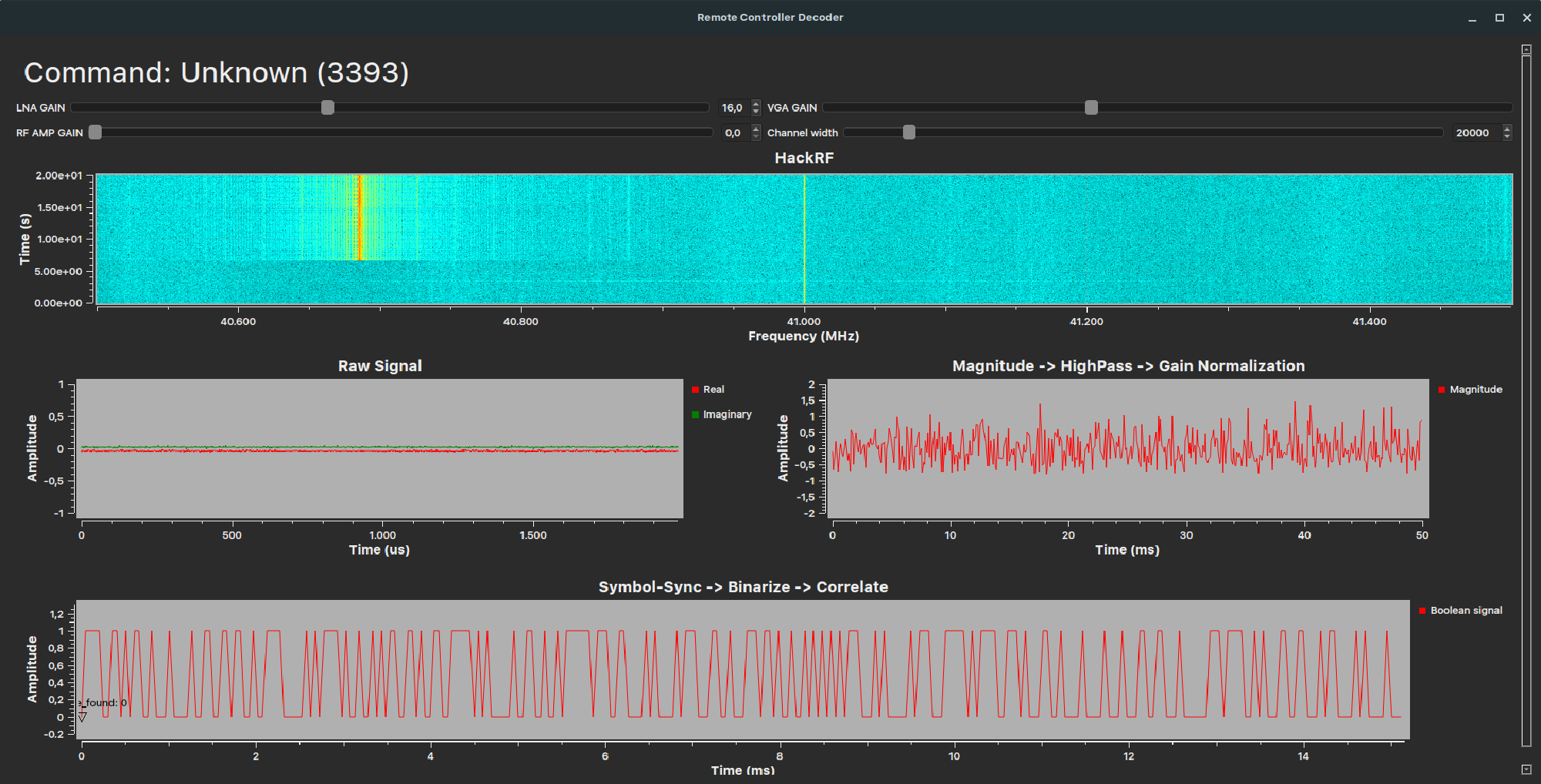
Chapter 7: Play computer games with the toy car remote #
To this moment, the GNU Radio provides info on which command is transmitted and when. It’s very cool to see the command decoding in real life!
Now how do we play computer games with it?
To control computer games, we need mouse, keyboard or gamepad input. Fortunately, this can be simulated using Python libraries such as pynput. My concept is:
- Modify the custom Command decoder Python-block in GNU Radio companion to set up a localhost UDP server and transmit the command strings over there. External applications on the same computer then can use the decoded commands to do more things.
- Another, external Python script is executed while GNU Radio is running, which:
- Acts as a UDP client, receiving the respective command strings
- Presses/releases keyboard keys virtually.
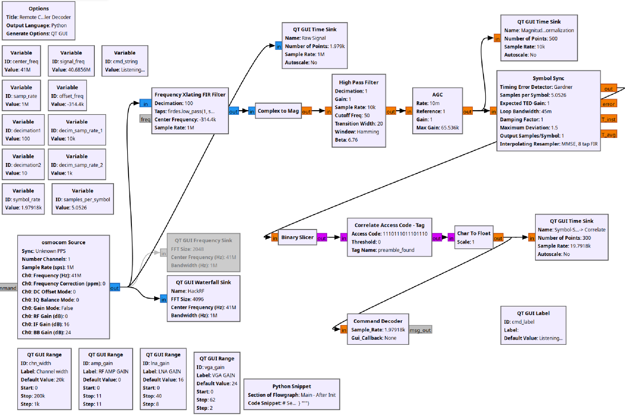
Result: The complete data flow & full demo #
We now have everything – from the toy car remote controller to the computer game. The following illustration shows the complete overview:
Let me show you the full demo, by:
- Starting and testing the GNU Radio processing pipeline
- Starting and testing the external, virtual keyboard controller
- Playing a computer game (in this case the old racing game FlatOut 2)
Conclusion & more ideas #
It’s possible to reverse-engineer a toy car remote controller and use GNU radio companion with some custom Python scripts to play racing games! I had a lot of fun to play around with the systems and concepts in this topic.
I learned a lot:
- How to use my HackRF with GNU Radio companion
- Some basics of RF modulation and signal processing
- Expectations for remote controllers in the future
And of course, the adventure continues! Having experience with a simple toy car remote controller enables me to do more complex projects:
Reverse-engineer an FM remote controller: I got an FM remote controller into my hands. I already started reverse-engineering it too. Since it is not as cheap and has a much better look and feel compared to the cars toy car controller, gaming with it on a computer is probably way better.
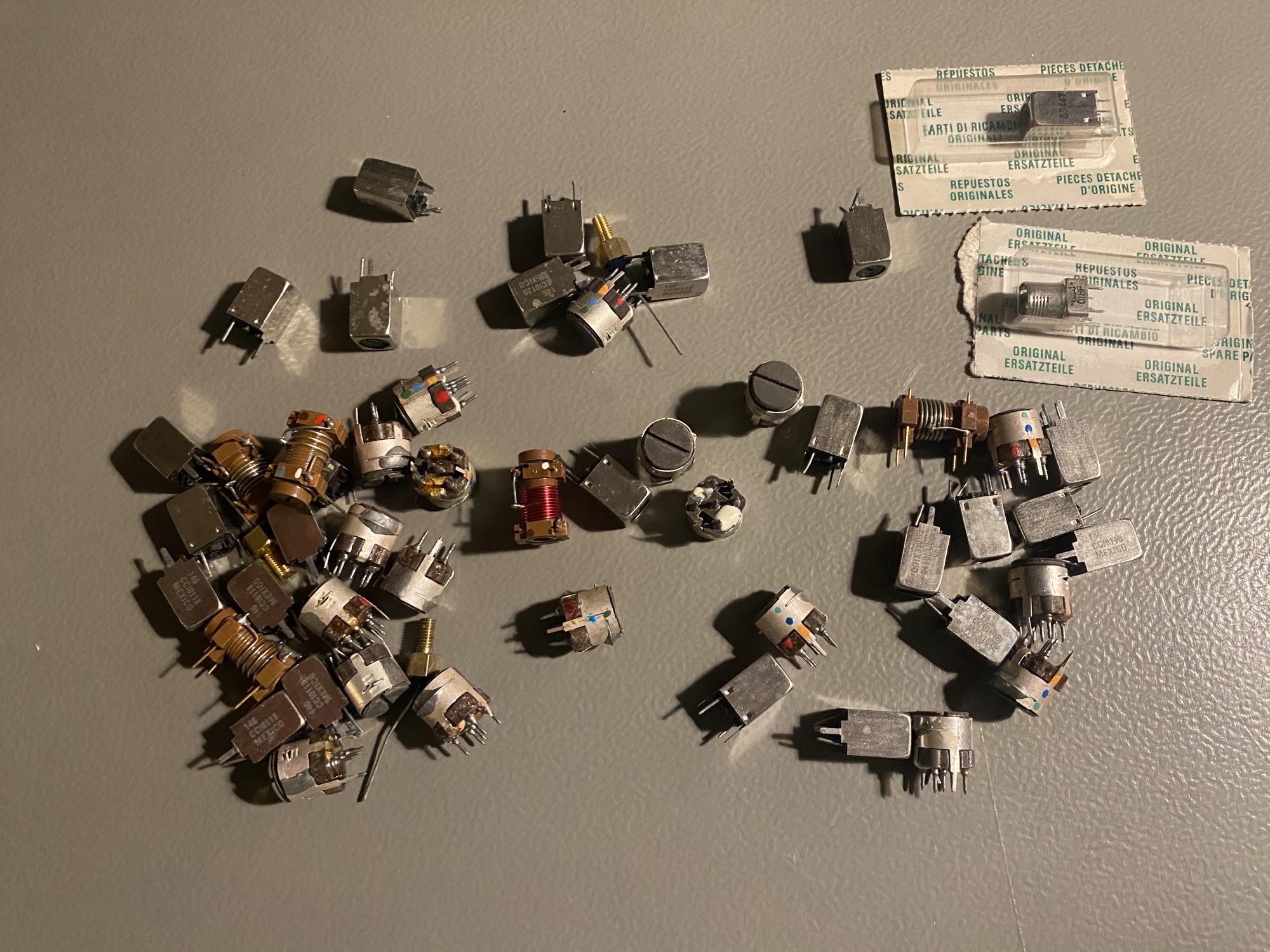
Building the command decoder purely in hardware: The latency of the real toy car and its remote controller is great in comparison to our custom decoder with the HackRF and GNU Radio (I don’t have objective measurements at hand). Building the decoder using analog hardware would significantly reduce latency. I already found some band pass filters in my cupboard that help detect the 40.685MHz signal from our toy car remote. Adding some comparators chips and an Arduino may be enough to build a full-fledged receiver!
Unfortunately not allowed: Steering the toy car with fake commands from HackRF The legal boundary is that we aren’t allowed to transmit with the HackRF since it is not certified like the original remote.
However, it’s possible to rebuild the remote controller in GRC to simulate signal:
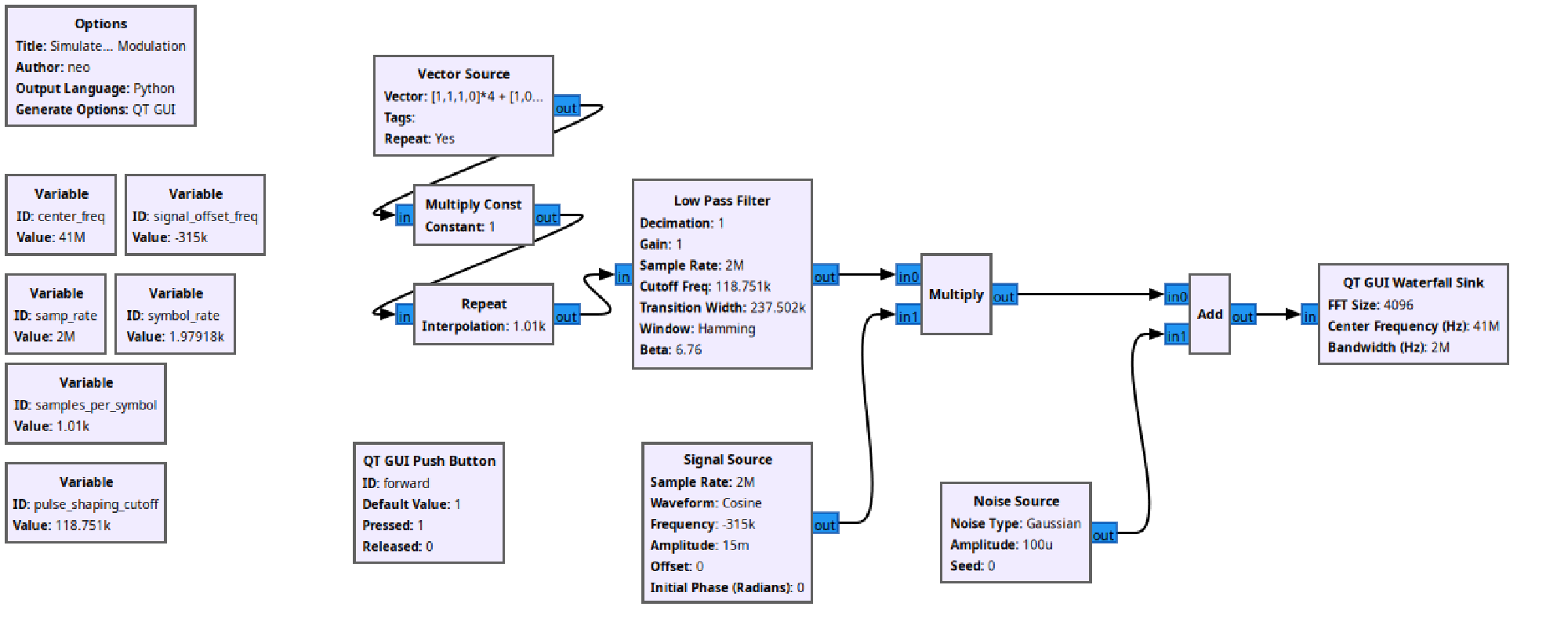
I am interested in your thoughts! - Reply with a simple Email
Have a nice day,
Carl
Attachments #
Attachment 1: The inside of the HackRF/Portapack #
To understand, what’s in my hands, we have to take the device apart:
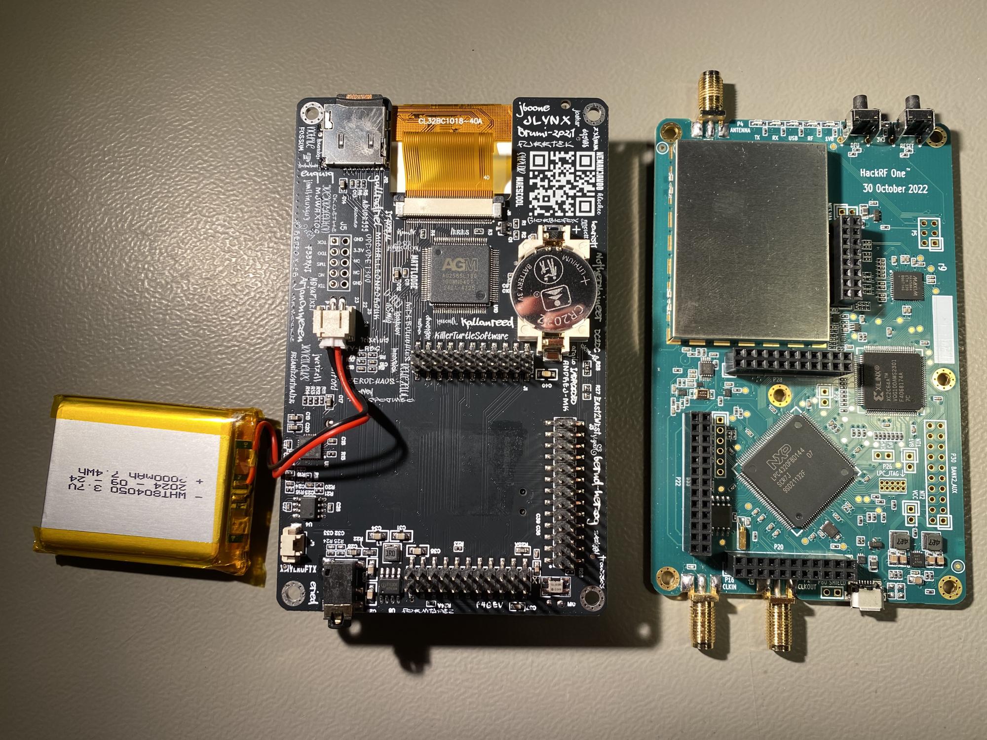
Actually, only the green circuit board on the right in Figure 39 is the HackRF. It’s the radio and decoding part. I guess I have a fake one, but it has the same functionality as the original.
On the left, the so-called Portapack can be seen. On the rear, it contains the screen and the buttons from the first picture. It has a small computer and a battery, which makes the HackRF portable! With it, a lot of functionalities are already provided like watching out for signals, receiving and decoding radio signals from airplanes and boats and simple listening to AM and FM radio music. Connecting the device to the computer removes any limits (needed for the toy hack).
Attachment 2: Inside of McQueen and the remote controller #
Taking apart McQueen reveals some juicy electronics:
The inside of McQueen #
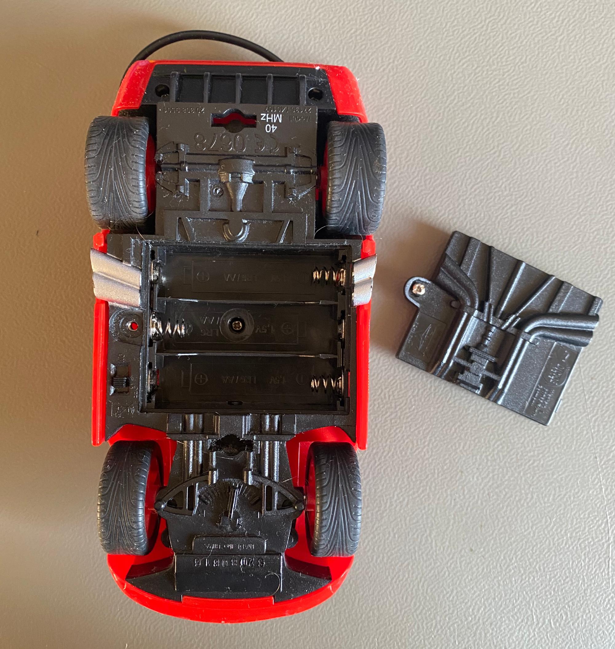
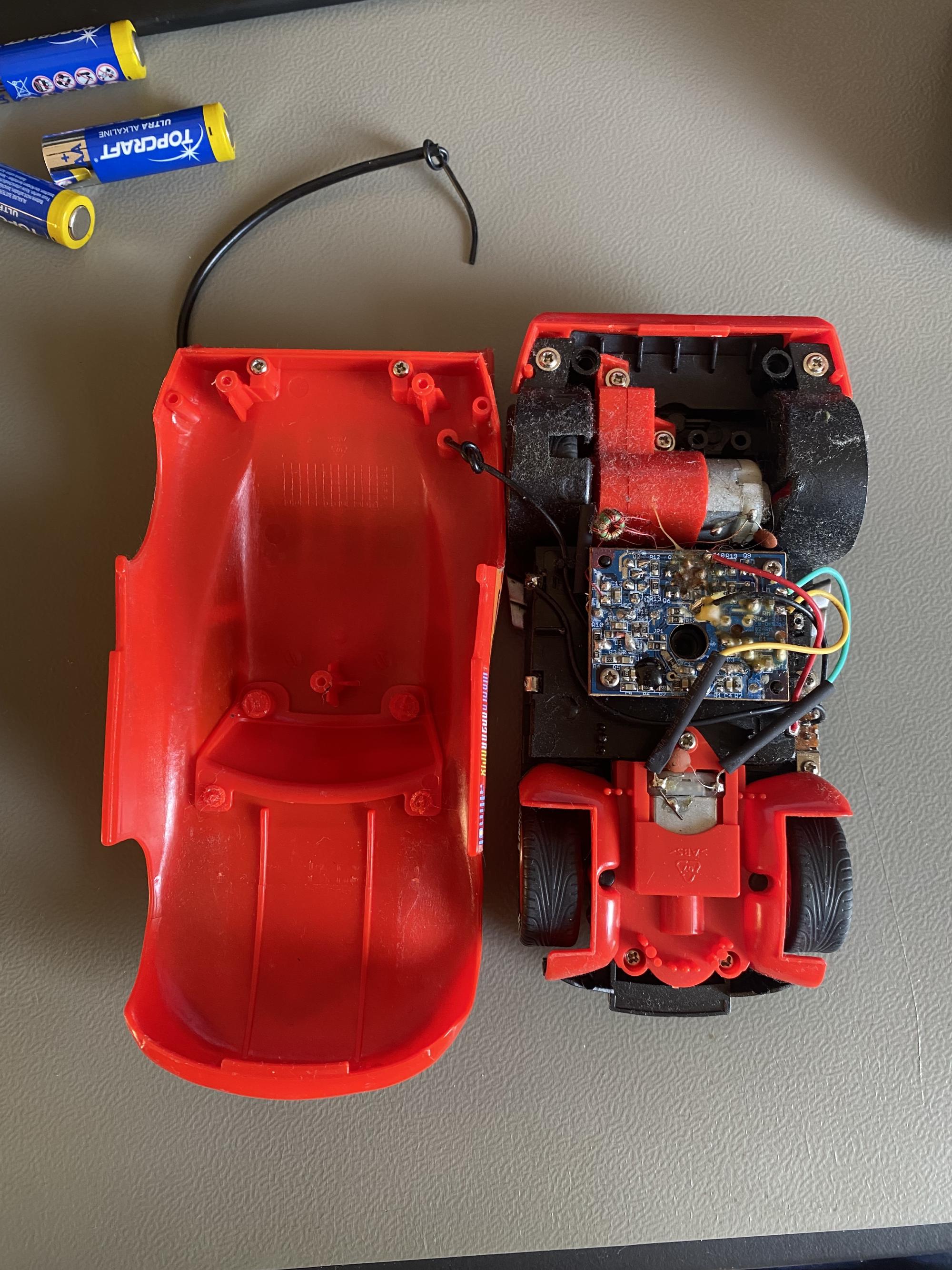
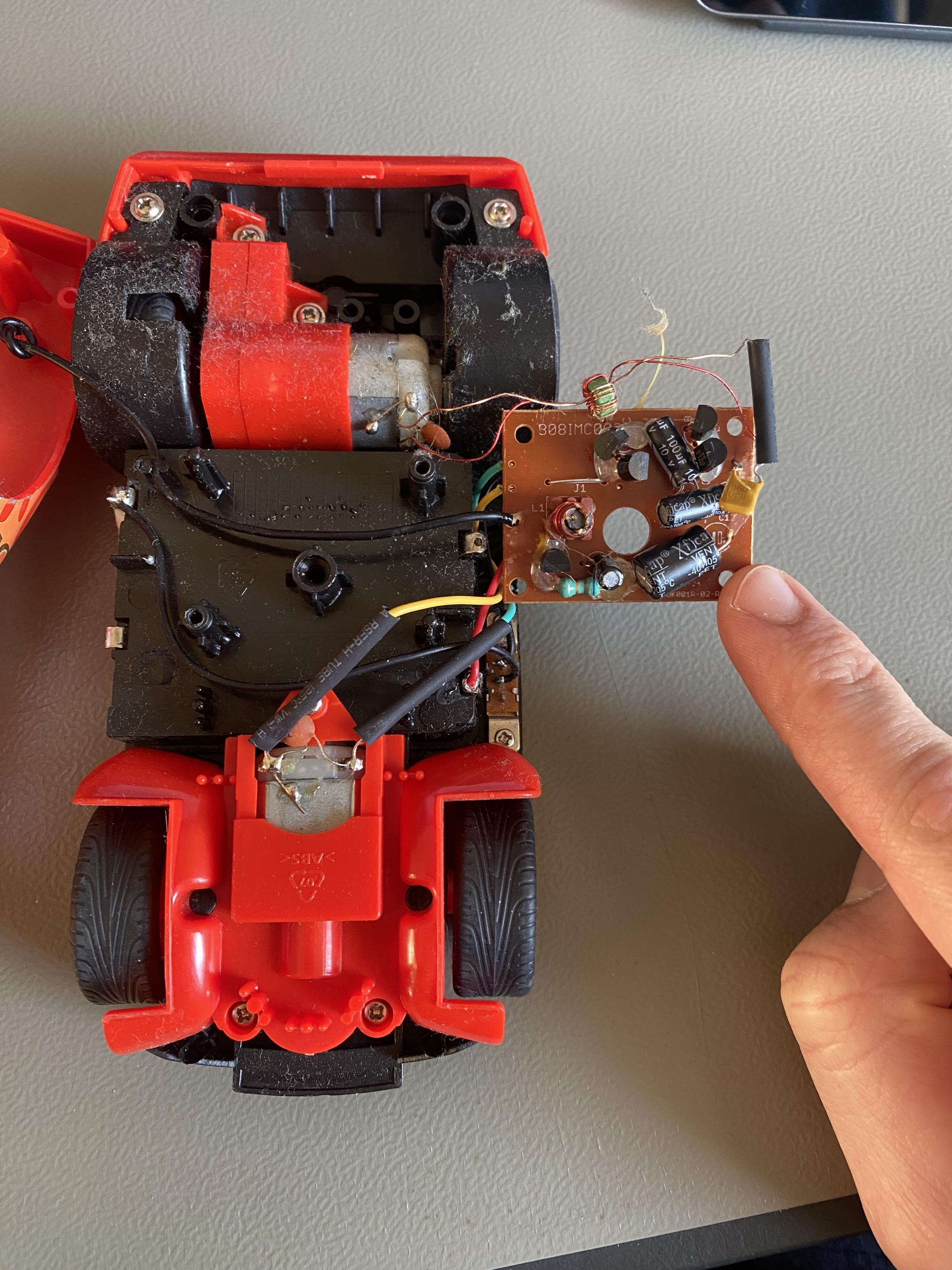
The most important info is the label “40MHz” at the bottom of McQueen.
McQueen consists of these parts:
- 2x Rear wheels connected to a motor which can go forwards & backwards
- 2x Front wheels, not connected to a motor, only for steering. It has a trimmer for fine adjustment
- Battery compartment for 3x AA batteries (so 4.5V in sum)
- Antenna (I guess a little more than 30 cm long)
- Controller PCB with batteries, motors & antenna connected to it
- On/off switch on the bottom
Initially, the antenna was broken, though functional. I fixed it by replacing it with a cable of matching length.
The inside of the remote controller #
Look, there is again another 40 MHz label!
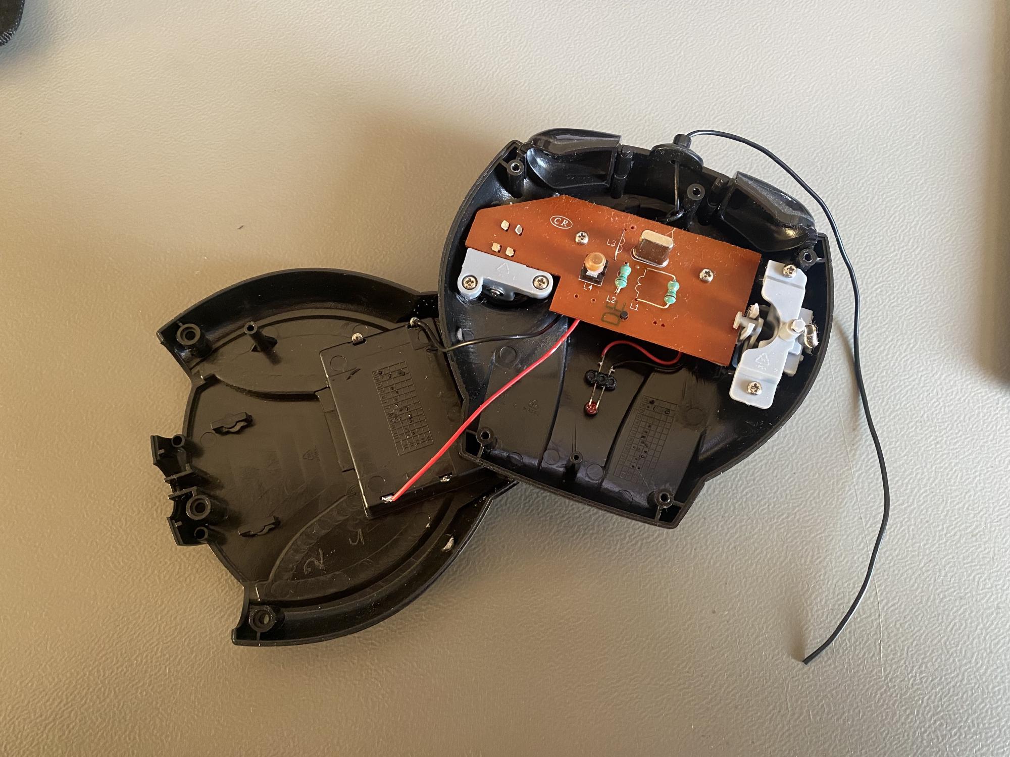
Next to the control sticks back sides, one can see a PCB with a crystal and several inductors on it.
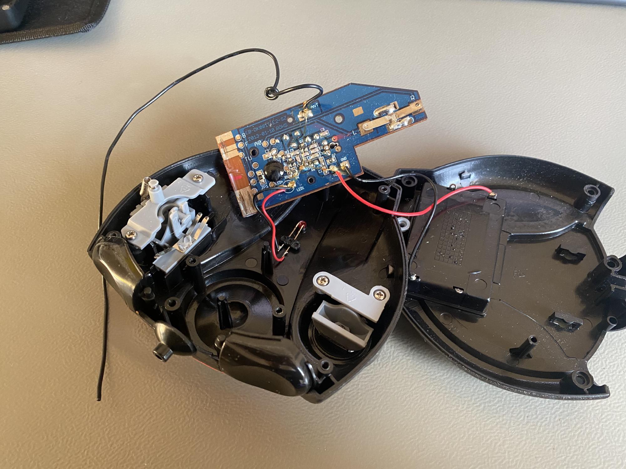
One can see the controller board with antenna, batteries and an LED connected to it.
The electronics of the remote controller consists of these parts:
- Two control sticks
- left sticks for gas: Four positions possible: Idle, backward, forward, forward with more speed. It’s not a continuous potentiometer
- right stick for steering: Three positions available: Idle, left, right. Also, no continuous potentiometer.
- Battery compartment for 3x AAA batteries (for 4.5V in sum)
- There doesn’t exist an on/off switch!
- LED indicating if the remote is currently transmitting
- Antenna (around 25 cm long)
- Controller circuit board